Numerical Modeling of the Mixing of Highly Viscous Polymer Suspensions in Partially Filled Sigma Blade Mixers (1)
1. Introduction
Attaining and ensuring homogeneity in particle-based slurries is not a trivial task—not least due to the complexity in quantifying homogeneity. The problem only gets more complicated when dealing with highly viscous non-Newtonian fluids. However, applications where homogeneity control is paramount are broad, extending to many industries such as food, pharmaceuticals, concrete and medical devices.
Some of the earliest attempts to obtain a quantification of homogeneity were made by Lacey in 1954 and later by P. V. Danckwerts. Both stated the importance of the sampling procedure, which is essential in determining whether particles in a population were evenly distributed. Other studies have used density as a method for the quantification of homogeneity. These approaches have used standard statistics methods such as Coefficient of Variance or Analysis of Variance (ANOVA). This works if you have appreciable unevenness in the distribution and a significant density discrepancy between components.
One of the pioneers within the field of mixing is Ica Manas-Zlaczower. Her famous dispersive mixing index from 1992 is still used today, along with her distributive Cluster Distribute Index. There have not been many alternatives to Zlaczower's dispersive mixing index. On the other hand, there are a number of alternatives to the Cluster Distribution Index—for example, the Scale of Segregation, a distributive mixing index that was developed back in 1952 and later applied in Computational Fluid Dynamics (CFD) models by Connelly and Kokini in 2007. Lastly, there is the Lacey mixing index, which has been modified over the years. Other indices that have been developed based on the Lacey mixing index include the Kramer mixing index and the Ashton–Valentin mixing index.
Heating is an important aspect of mixing, since it can reduce viscosity drastically. The advantage of reducing the viscosity is that it leads to an increased Reynolds Number, which improves mass transfer (i.e., mixing). The viscous dissipation of heat is a phenomenon that is often neglected in fluid dynamics. However, when dealing with highly viscous fluids, viscous heating can be present if they are mixed with a certain force. Consequently, this leads to an impact on the energy balance and should therefore only cautiously be ignored, as shown in previous studies.
Sigma blades can often be used as the rotating mixing element in a mixer when dealing with highly viscous fluids. They can be used either as a single-element or, as often seen, as a twin-arm mixer. Sigma blades have previously been simulated by Connelly and evaluated with respect to the dispersive mixing index. However, to the best knowledge of the authors, no numerical models have been presented in the literature that account for a free surface, a non-Newtonian material behavior and viscous dissipation when mixing with Sigma blades.
This paper presents a new non-isothermal, non-Newtonian CFD model for the sigma blade mixing of an adhesive suspension, where both the free surface and viscous heating are accounted for. The suspension is modeled as a viscoplastic fluid, and model calibration is performed via optical temperature measurements. To evaluate the mixing quality, we have used Zlaczower's dispersive mixing index as well as Kramer's distributive mixing index. The model is used to investigate the effect of applying heat both before and during the process on the mixing quality. The rest of the paper is organized as follows: Section 2 introduces the experimental setup as well as the numerical model, while in Section 3, the results are presented and discussed. Section 4 summarizes the conclusions of the study.
2. Materials and Methods
2.1 Experiments
The mixing material consists of a highly viscous polymer fluid and a multi-component powder blend. The powder contains both colloidal and microscale particles. The specific fluid/powder suspension is a piece of intellectual property and cannot be disclosed. The viscosity of suspensions changes with the volume fraction of the powder, but this is not accounted for in the numerical model, as it is assumed to have a limited effect on the results. The physical data, besides viscosity, are shown in Table 1. The density measurements were performed with a Sartorius YDK03 Density Kit for Analytical Balances, which uses the Archimedes principle. The heat capacity and conductivity measurements were performed on a TCi-3-A from C-Therm Technologies Ltd., which uses the Modified Transient Plane Source (MTPS) method that has been used in textile research.
Table 1. Physical data for the fluid.
| Name of the Property | Values | Unit |
| Density | 1133 | kg/m3 |
| Heat capacity | 1389 | J/kg·°C |
| Heat conductivity | k ( t ≤ 23 °C ) = 0.52 k (23 °C < t < 71 °C) = −1.88·10−3 t + 0.56 k ( t ≥ 71 °C) = 0.43 | J/m·K |
The experimental mixing was carried out on a Linden LK II 1 machine; see Figure 1. The machine has a mixing chamber with two sigma blades rotating in opposite directions. The front blade rotates at 60 rpm, and the one behind rotates at 19 rpm. Historically, this has been a typical setting for highly viscous mixing. The mixer also has a control panel to switch the rotation direction. In addition, there is a digital display that indicates the temperature, as measured at the bottom of the mixer. Attached to the mixing equipment is a heat exchanger that adjusts the temperature for the mixing process. A vacuum pump is also mounted to ensure that air is not trapped inside the mixture. Two walls in the mixer can provide heat to the system. If this function is on, the temperature will be 80 °C.

Figure 1. The mixing setup. (1) Chamber of the mixer, (2) control panel and digital display of the temperature, (3) heat exchanger, (4) vacuum pump.
2.2 Numerical Model
The CFD model simulates the mixing of the suspension in the mixing chamber and is developed in the commercial software FLOW-3D, which has successfully simulated other processes such as casting and 3D printing highly viscous fluids. An illustration of the mixer geometry is seen in Figure 2. At t=0, the fluid is well distributed at the bottom, and the powder is placed on top of the fluid. At t>0, the sigma blades start rotating. A no-slip boundary condition is applied on all solid surfaces. The computational domain is meshed with a uniform grid consisting of ~50,000 elements, which was arrived at after a mesh sensitivity analysis. The two side walls perpendicular to the sigma blades apply heat to the system; see Figure 2.

Figure 2. Illustration of the mixer geometry from (a) above and (b) the side. W and H have a distance of 120 mm, while L and u are 126.4 mm and 50.23 mm, respectively.
The flow is transient and non-isothermal since the viscosity is temperature dependent. The material is modeled as an incompressible substance, and thus, the density is approximated as constant. Hence, the flow is computed by considering the mass, momentum and energy conservation:

where ρ is the density, p is the pressure, k is the thermal conductivity Cp, is the specific heat capacity and q is the heat flux vector. is the material deviatoric stress tensor and is calculated as τ=2μ(γ˙,T)D. D is the trace of the deformation rate tensor, and it is defined as  . γ˙ is the shear rate and is calculated by
  . The gravitational acceleration, G, is given by
  . The software used the finite volume method to discretize the governing equations. The equation of energy is calculated explicitly, while the viscous stress and pressure are solved implicitly. The advection is solved explicitly with first-order accuracy. The free surface is calculated with the volume of fluid technique.
The material behaves as a non-isothermal viscoplastic fluid and is simulated by a modified Carreu model:

where μ0 is the zero-share-rate viscosity, μ∞ is the infinity-share-rate viscosity, n is the power exponent, λ is the time constant, E is an energy function which is dependent on the fluid temperature, a and b are empirical constants and Tref is the reference temperature. The applied values of the variables in Equations (5) and (6) are seen in Table 2. The shear rate-dependent variables are obtained via a rheological characterization of the fluid; see Figure 3. The temperature-dependent variables are obtained by a calibration, as the fluid was too viscous to perform measurements at low temperatures. The calibration is reported in Section 3.1.

Figure 3. Viscosity measurements compared to the model.
Table 2. Viscosity data of the simulated fluid.
| Symbol | Value | Unit |
| λ | 1 | s |
| n | −0.295 | - |
| μ0 | 4.35·108 | Pa·s |
| μ∞ | 2.9 | Pa·s |
| a | −20 | - |
| b | −95.2 | °C |
| tref | 20 | °C |
| γc | 1 | s−1 |
The evaluation of the mixing is carried out by a dispersive- and distributive-mixing index. The dispersive mixing is quantified through the Manas–Zlacower mixing index, λmz; see Equation (8). ω is the vorticity. When λmz is close to 0, the mixing is purely rotational driven, while at 0.5 and 1, the mixing is shear-driven and purely elongation-driven, respectively. The latter leads to a desirable faster breakup of agglomerates.

The second approach is a distributive mixing index where an artificial concentration or material is used. The concentration is defined as a scalar with zero diffusion, which does not affect the physics (such as the viscosity and density). Thus, the only effect is pure mixing. The mean of the concentration, c¯, is 0.5. The dimensionless concentration, ciˆ, and the dimensionless variance across the domain that contains fluid, S2, are found by Equations (8) and (9). From the variance, the Kramer dispersive mixing index, MKramer, can be found by Equation (10), where  and
and  , with P being the proportion of the component containing the concentration, which is set to 0.5 for this paper.

Table 3 presents the process parameters for the simulations that are studied in this paper.
Table 3. Information about the simulations.
| Simulation ID | Boundary Condition | Initial Condition | Simulation Time |
| CA23 | Adiabatic | 23 °C | 900 s |
| A23 | Adiabatic | 23 °C | 1800 s |
| A50 | Adiabatic | 50 °C | 1800 s |
| A80 | Adiabatic | 80 °C | 1800 s |
| NA23 | 80 °C | 23 °C | 1800 s |
| NA50 | 80 °C | 50 °C | 1800 s |
| NA80 | 80 °C | 80 °C | 1800 s |
© 2023 by the authors. Licensee MDPI, Basel, Switzerland. This article
is an open access article distributed under the terms and conditions of
the Creative Commons Attribution (CC BY) license (https://creativecommons.org/licenses/by/4.0/).