Mixing Performance Prediction of Detergent Mixing Process Based on the Discrete Element Method and Machine Learning (2)
3. Machine Learning Based Methodology
A machine learning (ML) algorithm based on multivariate polynomial regression (MPR) analysis was adopted to identify the relationship between variables and allowed the prediction of the mixing index.
The MPR used to estimate the coefficient values for different variables in the mixing process was derived from a Second Order Multiple Polynomial Regression expressed as:
where β1 and β2 are called as linear effect parameters, β11 and β22 are called as quadratic effect parameters, β0 is the bias, and ε is the error in the normal distribution.
According to [22], the Regression Function is given in Equation (2):
The representation of the polynomial regression in a matrix form is given in (3):
The estimated parameters can be computed as in Equation (4):
And the Computed Regression Equation is represented in (5):
In order to assess the accuracy of the predicted values obtained by the regression-based ML model, the most used traditional metrics can be adopted. MAPE (mean absolute percentage error), MAE (mean absolute error), RMSE (root mean square error), and R2 (coefficient of determination) metrics were calculated as in Equations (6)–(9):
where yi is the actual value,  is the predicted value, and n is the number of data points.
Figure 4 shows the flowchart of the methodology defined to predict the mixing index of the mixing process. The DEM model created is used to obtain the dataset. According the 25 design points listed in Table 4 and considering a time every 5 s from 5 to 60 s, a dataset of 300 data points was created. Each data point is composed by values of the inputs and the output. For the predictive model, the inputs are time and mass fraction of surfactant, carbonate, speckle and nonionic, and the output is the mixing index. The sulphate mass fraction is not considered an input because it depends on the total amount of the other components.
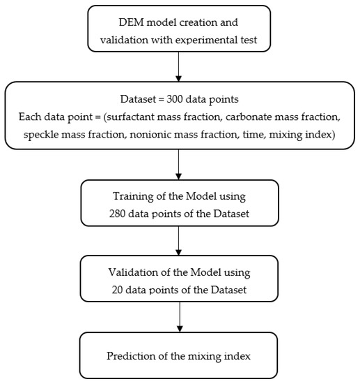
Figure 4. Flowchart of the methodology.
The dataset is divided into 2 parts. A total of 280 data points are used to train and test the predictive model. The other 20 data points are used to perform an independent validation of the model. In this process of training and validation, the accuracy of the predictive model results is assessed by calculating the error metrics indicated in Equations (6)–(9). Finally, the predictive model is obtained and allows us to predict the mixing index for any allowable combination of the components.
4. Results
The results show the validation of the DEM model compared with experimental results from a mixing test. In addition, the study of the effect of the initial component mass fraction and mixing time on the mixing performance is presented. The dataset acquired from this study was used to obtain a predictive model of the mixing index of the process that is also presented.
4.1. DEM Model Validation
To validate the DEM model, a mixing test with a 3D mixer was carried out and the mixture obtained from the test was used to determine the repose angle. The same procedure was simulated by the DEM model, and the numerical results were compared with the experimental ones. From a qualitative point of view, the mixing homogeneity was compared, and from a quantitative point of view, the repose angle.
The methodology consisted of filling the cup with the component mass fraction according to the formulation shown in Table 2, closing the cup with a lid, placing it in a 3D mixer and running for 60 s. In Figure 5 a screenshot taken during the mixing test is observed. Figure 6 shows the cup filled with the components totally segregated before the test, and the cup with the components mixed after the test.

Figure 5. Image of the mixing test performed in a 3D mixer.
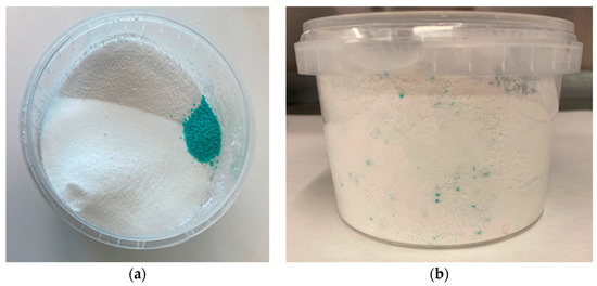
Figure 6. Mixing test. (a) Initial filling of the components in the cup; (b) mixture of the components after the mixing process.
Once the mixing process was finished, a sample from the mixture was taken to determine the repose angle by the fixed funnel method according to [24]. Figure 7 presents a comparison between the powder piles obtained from test and DEM simulation. From a visual perspective, it is observed that a high grade of mixing has been obtained in both cases. The repose angle test was repeated twice and both times the result was 32°, while a repose angle of 31.98° was obtained from the DEM simulation, as indicated in Table 5. Therefore, a great agreement between results from the experimental test and DEM simulation is observed.
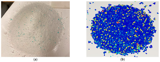
Figure 7. Powder pile from (a) experimental test and (b) DEM model.
Table 5. Comparison of repose angle between numerical simulation and experimental test.
| Repose Angle | Value |
| Numerical simulation | 31.98° |
| Experimental test | 32.00° |
| Relative error | 0.06% |
4.2. Mixing Performance Analysis
After validating the DEM model with experimental results, it was used to analyse the mixing quality as a function of mass fraction components and mixing time. To assess the homogeneity of the powder multicomponent mixture, a mixing index based on the pooled variance of the whole system according to the study developed in [25] was used, whose criteria is expressed in the following equation:

where M is the mixing index, σ2 is the unbiased sample variance of the concentration in a multicomponent mixture,  is the variance for multicomponent mixtures in the completely mixed state, and
  is the variance for multicomponent mixtures in the completely segregated state. All these variances are calculated by DEM simulation for a defined input dataset. The M index can take values between 0, completely segregated, and 1, completely mixed.
Every design point was simulated using the DEM model for a total mixing time of 60 s. The evolution of the mixture in the cup from the initial to the final instant of the process for the first design point is shown in Figure 8, where each represented instant matches with the end of a cycle of the mixer. A uniform mixing of particles is observed at 60 s from a visual point of view.
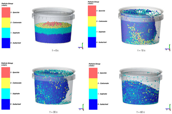
Figure 8. Simulation of design point 1 at different instants.
As time was defined as one of the input parameters, the M index output was obtained from DEM simulation every 5 s up to 60 s for all the design points, shown in Table 6.
Table 6. M index output for each design point at t = 5, 10, 15, 20, 25, 30, 35, 40, 45, 50, 55, 60 s
| Design Point | Time (s) | |||||||||||
| 5 | 10 | 15 | 20 | 25 | 30 | 35 | 40 | 45 | 50 | 55 | 60 | |
| 1 | 0.776 | 0.87 | 0.885 | 0.918 | 0.968 | 0.976 | 0.979 | 0.988 | 0.989 | 0.992 | 0.991 | 0.992 |
| 2 | 0.78 | 0.892 | 0.885 | 0.953 | 0.97 | 0.985 | 0.978 | 0.989 | 0.989 | 0.987 | 0.989 | 0.991 |
| 3 | 0.788 | 0.871 | 0.879 | 0.916 | 0.968 | 0.975 | 0.976 | 0.984 | 0.988 | 0.989 | 0.991 | 0.989 |
| 4 | 0.716 | 0.868 | 0.857 | 0.943 | 0.965 | 0.976 | 0.967 | 0.987 | 0.987 | 0.985 | 0.987 | 0.991 |
| 5 | 0.853 | 0.909 | 0.929 | 0.946 | 0.973 | 0.978 | 0.98 | 0.981 | 0.976 | 0.986 | 0.983 | 0.986 |
| 6 | 0.833 | 0.912 | 0.912 | 0.964 | 0.975 | 0.977 | 0.981 | 0.985 | 0.983 | 0.984 | 0.984 | 0.992 |
| 7 | 0.843 | 0.905 | 0.925 | 0.952 | 0.972 | 0.975 | 0.979 | 0.986 | 0.979 | 0.988 | 0.984 | 0.986 |
| 8 | 0.829 | 0.911 | 0.909 | 0.96 | 0.971 | 0.98 | 0.977 | 0.985 | 0.979 | 0.986 | 0.985 | 0.992 |
| 9 | 0.721 | 0.854 | 0.886 | 0.914 | 0.964 | 0.974 | 0.97 | 0.983 | 0.982 | 0.984 | 0.985 | 0.988 |
| 10 | 0.695 | 0.862 | 0.876 | 0.934 | 0.941 | 0.97 | 0.973 | 0.981 | 0.982 | 0.988 | 0.983 | 0.99 |
| 11 | 0.721 | 0.852 | 0.886 | 0.926 | 0.968 | 0.976 | 0.976 | 0.985 | 0.979 | 0.987 | 0.988 | 0.987 |
| 12 | 0.684 | 0.853 | 0.862 | 0.936 | 0.95 | 0.972 | 0.97 | 0.986 | 0.984 | 0.984 | 0.983 | 0.989 |
| 13 | 0.742 | 0.855 | 0.899 | 0.935 | 0.964 | 0.97 | 0.964 | 0.979 | 0.974 | 0.988 | 0.986 | 0.99 |
| 14 | 0.684 | 0.853 | 0.862 | 0.936 | 0.95 | 0.972 | 0.97 | 0.986 | 0.984 | 0.984 | 0.983 | 0.989 |
| 15 | 0.75 | 0.847 | 0.895 | 0.926 | 0.969 | 0.971 | 0.963 | 0.981 | 0.969 | 0.986 | 0.985 | 0.989 |
| 16 | 0.705 | 0.845 | 0.87 | 0.928 | 0.957 | 0.964 | 0.971 | 0.977 | 0.978 | 0.987 | 0.988 | 0.994 |
| 17 | 0.785 | 0.897 | 0.906 | 0.94 | 0.966 | 0.975 | 0.979 | 0.983 | 0.987 | 0.984 | 0.983 | 0.989 |
| 18 | 0.794 | 0.907 | 0.908 | 0.951 | 0.972 | 0.982 | 0.98 | 0.985 | 0.987 | 0.986 | 0.985 | 0.987 |
| 19 | 0.762 | 0.887 | 0.898 | 0.941 | 0.971 | 0.97 | 0.976 | 0.979 | 0.983 | 0.985 | 0.986 | 0.99 |
| 20 | 0.727 | 0.868 | 0.895 | 0.933 | 0.955 | 0.974 | 0.981 | 0.984 | 0.99 | 0.987 | 0.988 | 0.988 |
| 21 | 0.798 | 0.884 | 0.894 | 0.941 | 0.97 | 0.974 | 0.98 | 0.983 | 0.981 | 0.987 | 0.991 | 0.991 |
| 22 | 0.798 | 0.884 | 0.894 | 0.941 | 0.97 | 0.974 | 0.98 | 0.983 | 0.981 | 0.987 | 0.991 | 0.991 |
| 23 | 0.836 | 0.893 | 0.912 | 0.949 | 0.971 | 0.976 | 0.98 | 0.982 | 0.987 | 0.984 | 0.985 | 0.988 |
| 24 | 0.799 | 0.893 | 0.914 | 0.935 | 0.968 | 0.974 | 0.976 | 0.983 | 0.982 | 0.985 | 0.985 | 0.988 |
| 25 | 0.783 | 0.892 | 0.902 | 0.954 | 0.965 | 0.977 | 0.973 | 0.986 | 0.984 | 0.986 | 0.985 | 0.991 |
Figure 9 shows the variation of the M index with respect to time and the component mass fraction of surfactant, carbonate, speckle, and nonionic, where it was observed that the value of M index increases with time until it stabilizes at a value close to 1 in all cases analysed.
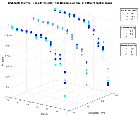
Figure 9. A 6D scatter plot of the M index depending on the inputs surfactant, carbonate, speckle, nonionic and time.
4.3. Predictive Model
The dataset of the powder mixing process obtained by the DEM model considering a defined range of every input variable, which are time and mass fraction of surfactant particles, sodium sulphate, sodium carbonate, coloured speckle, and liquid nonionic surfactant, was used to obtain a model that predicts the M index quickly and accurately from certain input values included in the ranges defined for them. For this purpose, a multivariate polynomial regression algorithm was used, which was trained and tested with 280 data points. After that, we validated the achieved model by means of an independent test dataset with 20 data points not used for training. The obtained model consists of the vector of coefficients used in the mathematical function, and is expressed in the following equation:

where M is the mixing index, xsurfactant is the mass fraction of surfactant particle, xcarbonate is the mass fraction of sodium carbonate, xsurfactant is the mass fraction of sodium sulphate, xspeckle is the mass fraction of coloured speckle, xnonionic is the mass fraction of liquid nonionic surfactant, and xtime is the time in seconds.
The error metrics obtained to evaluate the training and validation of the model are presented in Table 7.
Table 7. Error metrics
| Metric | MAPE (%) | MAE | RMSE | R2 |
| Training | 1.873 | 0.017 | 0.024 | 0.848 |
| Validation | 1.503 | 0.014 | 0.017 | 0.9072 |
5. Conclusions
In this work, the mixing process carried out by a 3D mixer for manufacturing a powder detergent was simulated using a DEM model, which was validated with experimental test. This computational model was used to study the mixing performance of the process considering mixing time and allowable mass fraction of components, at a mixer speed of 45 rpm. It was observed that a mixing index close to 1 was obtained in less than 60 s for all the combinations simulated, meaning that they were all completely mixed.
In addition, the proposed methodology based on DEM and ML to obtain a model which predicts the mixing index of the mixing process was developed. The DEM model was used to generate the dataset needed and a polynomial regression algorithm was used to obtain the model. It was demonstrated that the model predicts the mixing index of any allowable formulation with accuracy and in advance without requiring experimental test or numerical simulation. This method can also be used to optimize the mixing time necessary to obtain a uniform mixing of a defined formulation.
Cañamero, F. J., & Doraisingam, A. R. Mixing Performance Prediction of Detergent Mixing Process Based on the Discrete Element Method and Machine Learning. Applied Sciences, 13(10), 6094. https://doi.org/10.3390/app13106094
© 2023 by the authors. Licensee MDPI, Basel, Switzerland. This article is an open access article distributed under the terms and conditions of the Creative Commons Attribution (CC BY) license (https://creativecommons.org/licenses/by/4.0/).