Parametric Analysis of a Double Shaft, Batch-Type Paddle Mixer Using the Discrete Element Method (DEM) (2)
The input parameters are mainly adopted from the calibrated and validated model of Jadidi et al. . Moreover, a time step, , of 4.74378 × 10⁻⁵ s and a shear modulus, , of 1 × 10⁶ Pa were used for all simulations in the experimental simulation plan based upon a conducted stability analysis. The geometric properties are based upon the material stainless steel 304.
The simulation was started with a particle generation process called the filling process and the actual mixing process of the binary granular material. A static factory was used to randomly generate spherical particles with a downward velocity of 2 m/s (-Z direction in Figure 1). After a gravitational settling process for approximately 3 s, the particle bed reaches a steady state while the impellers remain stationary.
The steady state is defined as the moment when the particle bed reaches a kinetic energy/potential energy ratio equal to or lower than 1 × 10⁻⁶.
The number of particles follows from the input settings (particle diameter, composition and fill level). The mesh size is equal to 3Rmin. Thereafter, the shafts start to rotate according to a predetermined impeller rotational speed for 60 s.
To be able to assess the overall mixing performance of the system in a quantitative manner, a so-called mixing index is required. Typical characteristics of such an index include mixing process independence, ease of determination and accurate representation of the resulting mixing quality.
Bhalode et al. carried out a comprehensive review of different mixing indices available in the literature and classified them into three main categories, namely variance-based, distance-based and contact-based indices. Due to their simplicity, variance-based indices are most widely used to evaluate the mixer performance. However, they are highly dependent on the grid size of the system. A small grid size could overlook a sufficient mixture on a macro-scale level, while a coarse grid could miss micro-mixing effects. Therefore, in case a variance-based index is utilized, it is necessary to conduct a grid size analysis. The distance-based indices use the distance between particles belonging to different mixture components to measure the mixing quality of the (final) product. Although these indices are grid independent, they are computationally expensive and hard to implement compared to variance-based indices. Contact-based indices utilise the contacts of a singular particle with neighbouring particles to measure mixing. Although easy to calculate in DEM, these indices are impossible to measure in experiments and hence are not suitable for validation of the DEM model with experimental results. Additionally, in the granular dilute regime, where particles are far from each other in fluidized beds/zones, contact-based indices yield erroneous results.
As a result, the distance- and contact-based mixing indices are not suitable for this study since they are not only computationally expensive but also direction dependent and misleading in dilute regimes. Thus, the variance-based mixing indices are employed in the present study. According to Emmerink, all indices belonging to the variance-based set, excluding the mixing segregation index (MSI), are applicable.
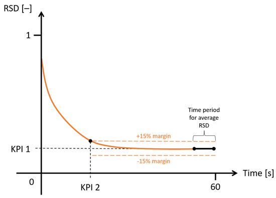
Here, the relative standard deviation (RSD) and Lacey’s index (LI) are used to assess the mixing performance of the system. These indices are frequently used and calculated by Equations (9) and (11). Theoretically, an RSD of one indicates a completely segregated mixture and an RSD of zero indicates a perfectly mixed mixture.

where is the standard deviation and is the average concentration over all evaluated bins. The standard deviation is calculated by Equation (10).
 (2)")
where and represent the total number of evaluated bins and the average particle concentration of bin , respectivelt. The concentrations in Equations (9) and (10) are defined as the number of particles of component 1 divided by the number of particles of component 2.
LI provides an indication of the mixture’s state as well but differs in definition. An LI of zero means a completely segregated mixture and an LI of one means perfectly mixed.

where  (2)") represent variances of the mixture where the subscripts and indicate a completely segregated state or perfectly mixed state. The variables are calculated by Equations (12)–(14).
represent variances of the mixture where the subscripts and indicate a completely segregated state or perfectly mixed state. The variables are calculated by Equations (12)–(14).

where is the average number of particles in a bin.
2.3 Plackett–Burman (P–B)
A two-level Plackett–Burman (P–B) was selected to conduct the design of experiments (DoE). The P–B design statistically examines the significance of factors and screens the most significant ones in the least number of runs, which is desirable due to the high computational time of DEM simulations. An N-run P–B design is suitable to study up to (N − 1) factors at two levels [36]. In this study, a 12-run P–B design was used to investigate nine factors as listed in Table 3. Besides the nine factors, two virtual factors (i.e., X1 and X2) were included to complete the P–B design. Altair’s HyperStudy v2022.1 was used to conduct the P–B design.
Table 3. Factors with corresponding levels for the Plackett–Burman (P–B) Design of Experiments (DoE).
| Factor | Description | Type of the Factor | Low Level (−1) | High Level (+1) |
| A | Particle size ratio | Material property | 1 | 3 |
| B | Particle density ratio | Material property | 1 | 20 |
| C | Composition (volume-based) | Material property | 0.25 | 1 |
| D | Initial filling pattern | Operational condition | FB | TB |
| E | Fill level | Operational condition | 60% | 140% |
| F | Impeller rotational speed | Operational condition | 40 rpm | 80 rpm |
| G | Paddle size | Geometric parameter | 0.67 | 1.5 |
| H | Paddle angle | Geometric parameter | 30 deg | 60 deg |
| I | Paddle number | Geometric parameter | 8 | 26 |
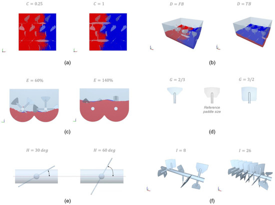
Figure 2. Illustrations of factor levels: (a) composition, (b) initial filling pattern (FB = Front-Back, TB = Top-Bottom), (c) fill level, (d) paddle size, (e) paddle angle and (f) paddle number.
Four key performance indicators (KPIs) were formulated to assess the mixing performance in terms of mixing quality, mixing time, average mixing power per kilogram and total energy consumption per kilogram. The LI outputs could not differentiate between the state of the mixing in twelve runs (i.e., LI values had a range of 0.84–0.99) and therefore, LI was not used for the analysis. Thus, four KPIs were formulated based on the RSD as follows:
4. KPI 4 (J/kg) Total energy consumption—Required energy to reach a steady state RSD.
2.4 Grid System
The RSD is highly dependent on the number of bins and bin size of the grid system. To select a suitable grid system for all twelve simulations, a grid system analysis was conducted on the worst-case situation, defined as the simulation run with the largest particle size and lowest particle number (run 5). The eight different grid systems are evaluated and shown in Table 4.
Table 4. Influence of grid system on KPI 1 for run 5.
| Grid Size | Cell Size Factor | Number of Bins | Average Number of Particles in the Bin | KPI 1 |
| 4 × 4 × 3 | 13 | 48 | 4288 | 0.099 |
| 5 × 5 × 3 | 11 | 75 | 2744 | 0.131 |
| 6 × 6 × 4 | 9 | 144 | 1439 | 0.134 |
| 7 × 7 × 4 | 8 | 169 | 1060 | 0.16 |
| 8 × 8 × 5 | 7 | 320 | 675 | 0.166 |
| 9 × 9 × 6 | 6 | 486 | 448 | 0.18 |
| 11 × 11 × 7 | 5 | 847 | 243 | 0.21 |
| 14 × 14 × 9 | 4 | 1764 | 117 | 0.258 |
A threshold value is determined to eliminate bins filled with particles lower than the average number of particles over all bins. The 7 × 7 × 4 to 9 × 9 × 6 grid systems yield approximately a 0.17 ± 0.01 (average) steady-state RSD. A lower or higher number of bins results in a higher deviation of 0.03. The 8 × 8 × 5 grid system maintains a sufficient balance between macro- and micro-mixing mechanisms and is therefore chosen as a suitable grid system.
2.5. Granular Temperature
The granular temperature indicates the mobility of bulk material in a certain control volume. The velocities of particles in any direction in a given time period are used to calculate this macroscopic characteristic as follows:
 (2)")
where u′ represents the fluctuation velocity of each particle at a given time and control volume and the triangular brackets 〈〉 function as temporal averaging within the control volume [4,10,38]. In general, the granular temperature is heavily related to the diffusive mixing mechanism of a mixing application [10]. A higher granular temperature means higher velocity fluctuations. In other words, particles behave in a chaotic and inconsistent way. To improve the understanding of the mixing mechanism in the paddle mixer and its relationship with the constructed KPIs, granular temperature data will be extracted from the DEM software. In this study, the granular temperature is used to provide further insights and support conclusions based on the KPIs.
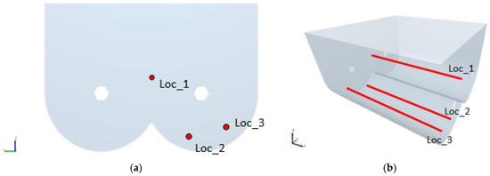
As the granular temperature is highly dependent on the control volume and the time step, a number of steps are conducted. The used DEM software provides granular temperature extraction from evaluation points. A distance-weighted sum of the particle data is performed using a normal weighting function, calculated by Equation (16), to obtain continuum temperature data between the evaluation points.

where ϕ is the normal distribution function and is the distance of a given particle from the evaluation point. The cut off distance identifies the width of the normal distribution function with a confidence interval equal to 99%. Alternatively, from a more practical point of view, the cut off distance is equal to the radius of the spherical control volume of one single evaluation point.
It is recommended to use at least a cut off distance equal to 9 times the average particle diameter in the system. To find a suitable cut off distance, the worst-case scenario is considered. Therefore, run 1 is chosen for finding a suitable cut off distance as this run consists of both particle diameters of 5 and 15 mm. For every run, a cut off distance of 25 mm is determined, where the evaluation points are a 2*cut off distance apart from each other. This comes down to a total number of 18 evaluation points over the length of the paddle mixer. To reduce the calculation time of each run, data are saved every 2 s. Consequently, a time step of 2 s was selected to obtain an average granular temperature over the full mixing period.